The Physics of Consciousness

The purpose of this post is to describe a simple analogy that communicates where the physics of consciousness can be found in the brain. The analogy given is one of an airport and the physics is the principle of flight.

Background

It is hypothesised that a simple, solid physical principle underlies consciousness. So far the hypothesis is that consciousness is a slow moving physical field that operates in the quasi static Darwin regime. That means consciousness is produced by electric fields, which further produce magnetic fields, but these magnetic fields do not produce transmitting fields. Further it is hypothesised that these fields produce consciousness in space-like spacetime. It is also hypothesised that consciousness occurs between action potentials. This means consciousness is produced by slow after hyperpolorization (sAHP) electric fields from ion channels. Starting with these ion currents the levels of consciousness are built up across the brain following the matrix described in this post.

Airports

Airports, just like brains, are complex as they contain many interacting complex systems such as roads, runways, hangars, terminals, car rental, maintenance, foreign exchanges, check-ins, security, departure and arrival boards, air traffic control, luggage, food, duty free, computers, customs, toilets, electricity and water.

So what is the physical principle underlying airports. Is it any of the functions, structure or processes involved in all the complex systems in the airport listed above? It’s none of them, it’s actually airplanes and more specifically its the physics of flight in the airplane wings. A very simple principle that if you had never seen anything flying would be very hard to conceive of.

If you were a blind researcher trying to understand how airports worked, you would find yourself in a very difficult position. You could analyse all the structures, functions, processes, intentions and purposes of the complex interacting systems and things in the airport and you would spend a long time understanding them. You could study the disruptions that occur if any of these systems fail. But you would be at a complete loss to understand what all these people were doing and why they suddenly vanished.

The physics of consciousness does not require an airport, a simple wooden glider being thrown can achieve flight, but you need to know where to look to find it.

Is Consciousness a space-like phenomena ?

The purpose of this post is to briefly describe how the electric and magnetic fields produced by slow moving ions in neurons creates a space-like spacetime that has the same nature as consciousness.

The hypothesis described in previous posts states that quasi-static electric and magnetic fields produced by slowly moving ions in confined water bound geometries can create super luminal fields with a space-like nature. This post extends this hypothesis by stating that conscious experience is formed by quasi-static, space-like fields in neurons.

The hypothesis is further extended with the working hypothesis that quasi static surfaces in space-like spacetime contribute to consciousness.

Extensions to the hypothesis further support the hypothesis that evolution has found an extremely energy efficient means to calibrate the brain by using superluminal fields that only transfers energy (material causality as force) when calibration is necessary.

Importantly a full treatment of the quasi-static fields in Maxwell’s equations predict that consciousness is space-like in nature.

Slowly Moving Ions

It is a misconception that the nature of electric and magnetic activity in the brain is either the production of electromagnetic fields or a sequence of static potentials. The brain’s activity related to consciousness consists of slowly moving ions, and only slow moving ions. Slowly moving ions do not produce electromagnetic fields in the form of luminal (i.e. light) fields, neither do they produce a series of static fields.

Slowly moving ions produce what are called quasi-static fields. Engineers call these quasi-static fields “approximations” because engineers use simplified versions of Maxwell’s equations when calculating them. This gives the impression that quasi-static fields are a second-class form of field. However quasi static fields are first class fields and actually have a more complex nature than both electromagnetc and static fields. The engineer’s approximation is a simplification of the calculations and not a simplification of the fields.

Understanding the electric and magnetic nature of fields in neurons is fundamentally about understanding the nature of “slowly” moving ions through neural geometries containing water. The starting point for this understanding is at there are a limited number of ions (e,g, Na+, K+, Ca+, Mg+, Cl-) and there are a limited number of channels and neural geometries through which they interact. Ions act as the source and target of electrical potentials and their movement is the source and target of electric and magnetic fields. Ions wavelength are in the visible spectrum.

Previous posts have shown the geometry of neurons mirrors the geometry of many electromagnetic nano technologies, such as waveguides, interference patterns, micro-spheres and nano-jets. It is significant that the geometry of both neurons and nano-technology is mirrored because the behaviour of electric and magnetic fields are geometrically scalable.

Recap – Quasi Statics in Water

The following section recaps previous posts on quasi-statics in water:-

1. Water forms a large majority of atoms in brain and all electrical signal must pass through it.
   
2. Bulk water has a permittivity of between 55 and 80 at body temperature already shows a low absorption to wavelength of 220. Water permittivity near some electrically charged surfaces reduces to 4-5 as the water adopts forms a structure.
   
3. A full treatment of quasi-static electric and magnetic fields in Maxwell’s equations have shown that fluxes can be “real”, “superluminal” and “space-like”.
   
4. Slowly, oscillating electric fields near the speed of brain wave oscillations, in confined geometries, reduce permittivity (ε) of water in the longitudinal and latitudinal direction to a value below one for a limited range of (ionic) wavelengths in visible light.
   
5. In the quasi static electric limit, when the permittivity (ε) drops below 1 then the quasi-static electric field becomes superluminal creating a space-like field. Similarly in the magnetic limit when permeability (μ) is below 1 then the magnetic field is super luminal creating a space-like field.
   
6. In the quasi static Darwin regime the electric field E is decomposed into the its transverse component ET and longitudinal component EL (Degond and Raviart 1992). When the transverse electric field is neglected, but not longitudinal electric field then fields are able to create feedback and thereby create internal oscillations but not radiation (Larson 2006).
   
7. This led to the following conclusion by Bauer 2018. “Prior to Maxwell there were two independent div[ergent] curl systems. In Maxwell’s equations there are two curl div[ergent] systems where the results of one feed into the source of the next. In Darwin there are three div[ergent] curl systems where the results fed into the next one.” (Bauer 2018).
   
8. In the quasi static Darwin limit longitudinal (flux) field is instantaneous. The overall (force) fields however are shown to not be superluminal (Kruger 2019). This implies that complex quasi static fields may be continually linked through non-radiative fields.
   
9. The four fields in Maxwell’s equations, can be categorised as either electric or magnetic and as with a force or a fluxes. Electric field intensity (E force) and magnetic field intensity (H force) are description of forces on the outside of a defined area that is essentially a conceptual black box. Electric current density (D flux) and magnetic flux density (B flux) are describe fluxes on the inside of the boundary that essentially form “conceptual” internals, which are actually real (LeBlonde 1973).
   
10. Oscillations in water by ions at slow frequencies reduces permittivity in confined water to create electric and Darwin quasi static fields, some of which could be space-like in nature. This allows the creation of complex div-curl systems. Faster oscillations create quasi static fields over longer distances.
    
11. Electromagnetic field theory creates complex surfaces, where fields form singularities. The hypothesis is that consciousness is dependent on these surfaces.
    
12. It is the hypothesis that the purpose of consciousness is to “calibrate” the brain in realtime. Calibration is meant ensure the quasi static fields in the brain interact to accurately reflect external representations. Evolutionary demands mean that energy, as force, is only expended when the brain needs to create a recalibration event or a reset event (action potential) in the control circuitry.
    
13. This leads to the hypothesis that complex divergent curl systems can be composed of slowly moving fields, and that when the permittivity is below one the flux fields are instantaneous, non-causal and create space-like fields.

Diagram (Kruger 2019) showing the quasi static limits. The hypothesis is that consciousness exists in and around the convergence of lines from quasi static (non-radiative) fields and is non-radiative, and space-like in nature.

Spacetime

A conclusion of the recap above is that consciousness exists in a space-like part of spacetime, in a complex quasi static div-curl system.

The modern study of spacetime in physics starts with with Einstein’s theory of relativity (1905) which led to Minowski’s 4 dimensional theory of spacetime (1906, 1909). In the past 50 years physics has used the theory of relativity and spacetime to explore the physics of black holes and the the big bang on a universal scale and quantum gravity on a planck scale. Space-like spacetime at the micro scale is relatively unexplored.

The intuitive understanding of 4 dimensional theory of spacetime has relied heavily on the idea of the light cone, where time is a vertical dimension, space is a horizontal dimension and an event occurs at the centre of the graph. The proportion of the graph is such that light (physical causality or force) travels upward at 45 degrees. Steeper than 45 degrees is time-like spacetime for events slower than light. Less than 45 degrees is space-like spacetime for events faster than light. space-like spacetime has, a four-dimensional non-Euclidean geometry (a sub-manifold)

Diagram (Minkowski 2008) showing the light cone, with space-like spacetime to the left and right of the event. The hypothesis is that conscious exists in space-like spacetime.

Space-like fields are hypothesised to form “maximal“ surfaces because the fields are instantaneous and time-like fields form “minimal” surfaces. This means fields in time-like spacetime form different topologies than time-like spacetime. The hypothesis is that quasi static (neuronal) topologies in time-like spacetime are rendered as different topological surfaces in space-like spacetime.

Recap – Phenomenal Experience

Conscious experience from a phenomenological perspective has been described in previous posts. Parallels between phenomenological conscious experience and theoretical space-like phenomena allows a rough topological mapping to be made. Phenomenological conscious experience gives a privileged insight into the nature of space-like spacetime. Previous posts have described how phenomenological theory has gradually developed to produce a body oriented continuous field, as follows:-

1. Brentano hypothesised consciousness was a unitary mental phenomena where intentional (directed) , non-atomic phenomena formed a spatial continuum. Every continuum consists of nothing but a continuity of boundary points.
   
2. Von Ehfrenal hypothesised the concept of a phenomenological field or “Gestalt“. Conscious thoughts are formed outside of consciousness and are temporal in nature. Temporal Gestalt are built up out of changes in non temporal gestalts in a unified manner, Foreground and background spatial shapes form the parts of a whole set against a background field.
   
3. Perls hypothesised consciousness happens at the boundary where a surface is adjusted between the organism and its environment so the field stays in equilibrium. When a field becomes tense or overworked it has excess energy and needs protecting. Consciousness is continually adjusting.
   
4. Merleau-Ponty hypothesised the simplest sensation is a dot-like figure on a background and forms a figure in a field. The body does not represent itself as a set of points in a space-time but the body implicitly includes this information, which is only later cognitively represented as objective spacetime points. According to Merleau-Ponty the visual field is not a bounded area, but folds around the body to create an experience of the whole situation, including quasi-visual elements.
   
5. Further Merleau-Ponty’s analysis of the Cogito is that it is a conscious act, whereby I think I am must itself be apprehended at the very moment at which it is carried out.

Note: A goal of the current hypothesis is to be able to implement (Marr 1982) the Cogito.

Spacetime and Consciousness

The hypothesis is that conscious phenomenological experience is space-like in nature. This hypothesis has been put forward already (Sieb 2016,2017), however the space-like hypothesis described here is derived from a complete treatment of Maxwell’s equations (LeBlonde 1973) which was referred to in earlier posts and provides a detailed physical theory of consciousness. The current hypothesis has described the time-like electrical aspects of neural topologies which are now assumed to map to phenomenological space-like topologies.

The space-like conscious hypothesis also addresses the Cartesian Dualism between mind and matter because space-like (mind) and time-like (body) spacetime form two regions with limited causality between them.

Consciousness phenomenological experience appears to form a continuum both spatially and temporally. That is to say small scale consciousness phenomenological experience appear within themselves to maximally occupy a space over time. A patch of colour or sound fully occupies its own spacetime.

At the smallest level conscious phenomenological experience appears to be contiguous both spatially and temporally. That is to say different spatial and temporal immediate conscious experiences appear to be absolutely contiguous but not merge or have a gap spatially or temporally.

Conscious phenomenological experience appears to form a figure and ground at larger scales. The figure and ground appear to occupy a space, but be separate. The hypothesis being that different figures in space-like space time can occupy overlapping spaces.

Conscious phenomenological experience appears to occupy the whole space at a larger scale. Space-like spaces occupy maximal surfaces because of their instantaneous evolution. Time-like spaces occupy minimal surfaces because they evolve through time and not space. Spatial and temporal conscious experience occupy the whole space in a maximal nature.

Broadly space-like phenomena can interact without having time-like causal effects. It is when permittivity goes above one that time-like causal effects occur. Phenomena in consciouness cannot have a direct causal effect on external time-like phenomena nor can external time-like phenomena have a direct causal effect on conscious phenomena.

Descartes Cogito and Descartes Dualism can also be analysed from a spacetime perspective, The space-like nature of spacetime creates an instantaneous field where parts field are available to other parts of the field. Space-like maximum occupation provides a continuity that gives the Cogito its certainty. The causal relations between matter and mind can be reinterpreted as the relation between time-like and space-like phenomena. Time-like phenomena are materially “causal”. Time-like phenomena interact with space-like through field interactions.

The ability to reduce the permittivity of water, using oscillations for a narrow band of ionic wavelengths, creates a controllable “spacetime bridge“ (a conscious bridge) across neural geometries, with the same physical function as Descartes meta-physical pineal gland.

The geometry of the brain and consciousness appear at first to be very different and related in a complex way. In space-like spacetime geometry is not the same as time-like spacetime geometry. The mapping between space-like and time-like geometry (sub-manifolds) is explored in topological mapping theory. For example spatially tree structures or chiral structures in time-like geometries can map to complex surfaces in space-like geometries.

In one sense space and time reverse in consciouness. In consciousness a thing appears to hold phenomenological time if it occupies a space, and a thing appears to have phenomenological space if it occupies time. That is to say the phenomena of space and time is the conscious experience of time and space.

Conclusion

It is not just that space-like spacetime shares characteristics with phenomenological consciousness it is that quasi static fields and and the brains biochemistry of slow moving ions and oscillating water predict space-like phenomena as the basis of fields of consciousnesses.

In the “matrix“, presented in a previous posting, the subjective (mind) perspective is now hypothesised refers to space-like phenomena and the objective (matter) perspective refers to time-like phenomena. Language refers to our ability to independently refer to the activity of space-like and time-like phenomena.

The space-like conscious hypothesis offers a solution to the mind-body problem by proposing the mind is space-like in nature where the body is time-like in nature, and that casual relations are between mind and brain is based on the evolutionary function that consciousness provides real-time calibration in the brain.

Consciousness is a robust and reliable system that represents the environment in realtime and calibrates the organism to its environment. It is also a requirement that this system of calibration is efficient. To be evolutionary advantageous the organism has discovered a payoff between objective, time-like (materially) casual advantages and subjective space-like non-(materially) causal advantages.

Future posts will look at original work on space time and and other topological analysis of spacetime. In particular how spacetime topologies, space-like surfaces and quasi static field geometry relate to consciousness.

Simple Images in Y-Junction waveguides

 

The purpose of this post is to very briefly describe how waveguides can transmit Waveguided “images” in Y-Junction waveguides fields, such as Gabor waves.

Transmission Efficiency

Waveguides can carry a number of different “modes”, which depend on the wavelength, diameter, boundary and permittivity of the channel. Previous posts have shown that neurons could carry modes for various ions.

A problem with transmitting complex images along a waveguide is that the image will degrade rapidly due to a phase delay in higher modes in the waveguide (Feshchenko 2003). In otherwords higher modes curl more in the waveguide which slows down the wave relative to faster modes.

In order to overcome the limitation of mutiple modes research was undertaken trying to bypass this limitation. Complex waveguides were produced, which either modified the phase velocities of different modes or encoded images in a form that could be passed efficiently (Feshchenko 2003). If an image is transmitted as its Fourier transform then the image can be transmitted without loses, because the modes of a waveguide are eigenfunctions of a Fourier transform (Df=λf).

Few Modes

The current demand for network bandwidth has meant single mode optical fibres can no longer keep up with demand. This has led to a lot of interest in developing optical fibres that can carry multiple modes (Riesen 2013).

The problem with large diameter fibres is they can transmit a lot of modes which suffer from interference, phase velocity conflicts and modes degenerating. To overcome this researches have developed “few mode fibers” (FMF) where only a limited number of modes are available (Wang 2014).

Diagram (Riesen 2013) showing some modes that could be transmitted down a fibre.

Few mode transmission have been shown to be efficiently transmitting over 1000s of Km (Yaman 2010)

Diagram (Bali 2012) showing the intensity patterns after 50-km in a few mode fibre (Bai 2012)

It’s important to distinguish the form of the mode from its contents. Whilst the form of the mode (TE/TM) has a geometry (see above), the content of the mode could be the intensity within the mode. In the simplest case the geometry of mode represents the information. If the content of mode is a simple field, such as a Gabor wave, it can be carried efficiently.

Splitting Waveguides

Y-junction waveguides can be used to split and combine modes.

Diagram (Saleh 1991) showing the mode splitting

The output is split between each channel, so in the case above 50% of the output would go through each output (Syms 1992)

Diagram (Syms 2992) showing a wave splitting.

Splitting can be scaled up to multiple branches.

Diagram (Guider 2009) of a 1×8 waveguide splitter showing two modes being carried, with TM the mode being carried more efficiently than the TE mode.

To filter different modes through different channels several techniques have been used. These include changing the diameter of each of the output channels so that different channels support different modes.

Combining Waveguides

As well a splitting modes Y junctions can be used to combine modes. The output of combined modes depends on the position of Y junction as to whether there is constructive or destructive interference.

Diagram (Saleh 1991) showing modes combining.

Diagram (Saleh 1991) showing two modes and a combined mode

Waves in Y-Junction splitters and combiners can either transmit all the energy or none of the energy. When combining fields no losses occur when both inputs phases and amplitudes are equal, but all power will be lost if both inputs are excited and out of phase. When splitting fields the energy will be split if the outputs can carry the same mode. In the situation where the waveguides narrow below the cut off limit then power will be lost.

Diagram (Syms 1992) showing when two modes are combined the input fields are summed as a super-postion. If all the inputs have equal amplitude and phase then the output it 100%, or if they are oppositional it could be 0%.

A Neural Perspective

From a neural perspective Y-Junctions waveguides bare a similarity to dendritic trees.As dendrites change in diameter along the length of the dendritic tree this would cause the modes to change or be eliminated unless the permittivity of the water also changes to maintain the waveguides above the cutoff wave length. The limited ion wavelengths available mean few modes could only ever be carried.

Energy can be carried by transmitting waveguides modes or reactive near fields. However moving ions produce quasi static electric fields that can carry reactive fields and energy with both limited divergence and curl.

Do Spines couple like Microspheres on Waveguides ?

This post is the second of several that explore the possibility that dendritic spines and dendritic branches function like microspheres and waveguides used in nanotechnology. The purpose of this post is to explore the simlarlies between nanotechnology of microspheres coupling on a waveguide and spines coupling on a dendritic branch.

The previous post described how dendritic spines might produce a nano-jet that passes through the spin neck into the dendritic branch. The previous post also touched on how microspheres are used as sub-wavelength lenses to either enlarge or shrink images. Previous posts have also explained how neurons can act as waveguides and have a dieletric constant of less than 2 required for microspheres when water is oscillated.

This post takes this further by hypothesising that local spines on the same branch might couple. Interestingly I cannot this hypothesis in any literature.

Coupling to a waveguide

The term “coupling” means how fields interact between a microsphere and a waveguide. The physical process of coupling is achieved by superposition. The coupling to or from a microsphere or waveguide, whether or not the field is near (evanescent/reactive) or far field (planar/transmittive) is done by evanescent fields.

A number of different mechanisms have been used to couple microspheres to waveguides. Each of the different mechanisms have different characteristics (Little 2000). For example, the prism coupler is efficient but bulky, and has poor waveguide characteristics. The tapered optical fibre is efficient but fragile. The half block coupler is robust but inefficient. The hybrid fibre-prism is efficient and can act as a wave guide.

Diagram (Little 2000) showing a number of ways of coupling microspheres to waveguides.

The previous post examined whispering gallery mode (WGM) microspheres. Whilst it is not hypothesised that spines are WGMs they can be used to demonstrate some coupling characteristics. Whispering gallery microspheres can be coupled to a waveguide by placing a tapered optical fibre waveguide next to the microsphere. This is because tapering thins the waveguide and creates an evanescent field outside the waveguide, and it is this part of the field that can tunnel into the microsphere. The thinner the waveguide, larger the evanescent field outside the waveguide, and the stronger the coupling.

Diagram (Kippenberg 2004) showing how light passing down a waveguide is coupled evanescently to a microsphere.

Evanescent coupling using a tapered waveguide is efficient and can couple up to 99.9% of light (Spillane 2003). However this method is too fragile, labor intensive and subject to environmental conditions to be of practical use (Murugan 2010).

The efficiency of the coupling can be varied by adjusting the distance between the microsphere and waveguide.

Gorodetsky (1998) observed efficient coupling is a function of both the distance from the waveguide and the wavelength.

Graph (Gorodetsky 1998) showing the coupling efficiency based on wavelength and distance. Note: graph shows amount of energy not passed into the sphere from the waveguide. When coupling occurs the graph drops.

Gorodetsky (1998) also noted that near-field evanescent coupling may be not a unique method to efficiently excite modes in microspheres. For example feno resonance or the scattering of radiative modes could have an effect.(Shashanka
2006).

Whispering gallery mode microspheres resonate at different wavelengths, implying microspheres with different sizes can resonate at common wavelengths.

Diagram (Murugan 2010) showing how WGM microspheres have different resonant wavelengths and whose strength varies with separation from the waveguide.

Coupling microspheres along a Waveguide

The next section briefly describes the situation where multiple microspheres exist on the same waveguide. The dynamic geometry of the fields in the microsphere and waveguide are called modes. The microsphere is called the resonant mode and the waveguide the guided mode. The theory is that multiple resonant modes can couple to the guided mode.

Serpenguzel (2011) showing how two microspheres can exist on the same waveguide. The similarity to dendritic spines is obvious.

Xiao (2008) analysed the coupling between two whispering gallery mode microcavities via a coupled fiber taper. The efficiency of the coupling with the coupled microcavities can change dramatically depending on the wavelength and this leads to a steep narrow transmission peaks between the waveguide and microcavity at certain wavelengths.

Resonant coupling between microspheres has been found for glass microspheres, on a chip with photonic crystals (Xiao 2008). The efficiency of the coupling is based on the distance between the microspheres and the wavelength, and the permittivity of the microspheres which changes the whispering gallery resonance. The coupling strengths between the waveguide and the cavities could be controlled by adjusting the air gap between the microsphere and the waveguide.

Xiao (2008) showing two whispering gallery microspheres and the flow of the field.

Heebner (2002) coupled multiple microspheres on a waveguide and managed to “slow” the light down when light fills up the cavities. The direction of the flow of the down the waveguide determines the direction of the light in the whispering gallery mode in the microsphere. When the light flows into a microsphere it eventually saturates the sphere causing the field to then flow into the next microsphere which is then in turn saturated. In this way the microsphere acts as a capacitor and slows down the flow of the field.

Xiao Y-F, Min B, Jiang X, Dong C-H, Yang L. 2008. Coupling Whispering-Gallery-Mode Microcavities With Modal Coupling Mechanism

Heebner (2002) showing multiple microspheres on a waveguide.

Yanik (2005) coupled cavities on a waveguide and found direct coupling due to photon tunnelling between the two cavities.

Diagram (Yanik 2004) showing how multiple cavities can be evanescent coupled along a waveguide and the coupling decreased exponentially with the distance between the cavities.

So far the light has been “reciprocal”, in the sense that when one microsphere fills up so does the next and so on. Control on whether the light enters the waveguide is based on the distance the microsphere is from the waveguide, the resonant wavelength of the microsphere and whether the microsphere is saturated.

In spines the control over microspheres distance from the waveguide would be mirrored by changing the length and diameter of the neck. In addition saturating the microsphere would be mirrored by filling the dendritic spine with ions. Changing the neck length (Arayaa 2014) and spine shape (Fischer 1998) is known to take place over minutes, whilst saturating the spine with ions is known to take place over milliseconds.

Resonance around a circuit

A second channel on a series of micro-resonators enables the field to create feedback. In the case of whispering galley modes when the wavelength of a resonator is an integer of 2πR it creates resonance. When the distance between the micro resonators is an integer of 2D the two resonators both absorb the wavelength. When the resonators have a feedback loop via a second (drop) waveguide then constructive interference occurs through the drop waveguide and a phenomena known as coupled resonator induced transparency (CRIT) occurs.

Diagram (Guider 2009) showing how (a) a whispering mode gallery sends the wave into a reverse wave guide on one resonant microsphere (b) how whispering mode gallery sends the wave into a reverse wave guide on more than one resonant microsphere and (c) how the resonant wavelength between microspheres creates coupled resonator induced transparency.

The phenomena of coupled resonator induced transparency (CRIT) will be examined in more detail in a later post.

Coupling in Spines

Electrical activity in spines has been found to cause electrical activity in closely positioned spines on dendritic branches (Lee 2016). Using fluorescent calcium indicators it was shown (Lee 2016) that electrical activity from one spine spread to create electrical “hotspots” of 100um along a dendrite which moved into the spines. This activity lasted over 1000ms. This electrical activity was created by local amplification of calcium from within the spines and dendritic branch.

Picture (Lee 2016) showing fluorescent calcium indicators in dendrites.

Picture (Lee 2016) showing fluorescent calcium indicators in dendrites.

The long lasting signals (Lee 2016) were found in dendrites during development. This indicates that electrical coupling between dendrites is important during development. In contrast, adult cells also produce large calcium signals that occur in dendrites and last a much shorted duration of 200ms (Sabatini 2002). The hypothesis is that during development electrical coupling last longer and is used to align the geometry of the spines, but during adult consciousness the signals are shorter and reflects the activation of electrical patterns. The hypothesis is that coupling during development aligns the spines, whilst coupling during adulthood maintains this alignment through calibration.

Dynamic Changes in Coupling

Spines are dynamic over periods of minutes and somewhat unique. No spine looks quite like any other (Tønnesen 2010). There is a broad distribution of geometry, where spine head volumes vary between 100nm and 1000nm, spine necks diameter measures between 50nm and 500nm and their length measures between 100nm and 3000nm.

Tønnesen (2010) observed that adjacent spines do not look like each other. This may have an impact of spines coupling via the dendritic branch. If it assumed identical spines on a dendritic branch couple more easily and that spines resonant properties couple more easily, then spines that are different are less likely to couple. For example adjacent spines on a dendritic branch may need to modify themselves in order to couple.

Diagram (Tønnesen 2010) show a diverse range of spine shapes and sizes.

Diagram (Tønnesen 2010) showing how adjacent spines look different. And have different activation profiles.

Spines change their shape in response to a variety of triggers, including long term potentiation (LTP) and depression (LPD). The change in shape of the spine (head diameter or shape, or neck diameter or length) accounts for more than half the electrical activity (Tønnesen 2010), as measured by fluorescent activation. Other causes of activity could be changes in the spines internal skeleton, changes in ion channels or changes water permittivity during oscillation.

Over half the intensity of activation of a spine (Tønnesen 2010) can be calculated from the following formula, where V is the spine head volume, L is the spine neck length, A is the spine neck cross section and D is the diffusion rate.

τ= ( V x L ) /( A×D )

This equation shows that changing the geometry (numerator or denominator) of the spine may be additive or may cancel out changes in the the electrical intensity (Tønnesen 2010) whilst also changing other properties. For example if the head becomes larger and the neck becomes wider the activation time in the spine may stay constant, but the activation intensity may increase. Similarly the activation time may increase and the activation intensity stays the same. This allows a spine to tune its electrical behaviour.

Diagram (Tønnesen 2010) showing a spine changes , over a few minutes showing the activation times change but the intensity stays constant.

Tønnesen’s (2010) observation that adjacent spines differ in morphology may depend on which part of the dendrite is being observed. For example, Morales (2012) found a random distribution of spines in dendritic branches midway along the dendrite, where small spines occur more commonly in pairs than large spines. Distal and proximal dendrites have clusters of spines.

Non reciprocal coupling

Coupling in the context of this article refers to coupling between microspheres and waveguides, or spines and dendritic branches. When identical microspheres are connected perpendicularly to waveguides then directional coupling is reciprocal. That is fields entering the spine from one direction of the waveguide enter as easily as fields from the other direction. A form of non reciprocal directional coupling was discovered by (Peterson 2018) where coupling between the guided and resonant modes of whispering gallery modes only happens when electrical fields come from one direction.

Peterson (2018) discovered where whispering gallery cavities do not have symmetry (i.e. they are chiral) then directional coupling can be non-reciprocal. In other words coupling is different in a clockwise (CW) and counter clockwise (CCW) direction. Any cavity with a small deformation can be non-reciprocal. Some micro cavities showed strong counter- clockwise (CCW) coupling but weak clockwise coupling (CW).

Diagram (Wiersig 2011) showing asymmetric whispering gallery mode.

These asymmetric cavities, are called Gutkin’s cavities, where at any point at the boundary the maximal distance to other points of the boundary is a constant. It would be possible for spines to internally adjust their internal actin skeletons to form Gutkin’s cavities in order to calibrate themselves.

Diagram (Wiersig 2011) showing a Gutkin cavity.

The diagram above (Wiersig 2011) showing the difference in coupling by asynchronous cavities when electric fields propagate in clockwise (CW) and counter-clockwise (CCW) directions.

The symmetry of the cavities also has an effect on the direction of the nanojet outside the cavity. In neurological terms this would mean that asymmetric spine heads would be correlated with the direction of the spine head on the spine neck.

Diagram (Wiersig 2011) showing how asymmetric cavity creates directional nano-jets

Discussion

The post has looked very briefly at the how microspheres might be coupled via waveguides. Coupling of spines via dendrites raises specific points and questions about fields inside dendrites.

An important point is that when local spines couple if the synapses contain electrical synapse clusters then two other neurons couple together for a brief moment in time like an old fashioned telephone exchange.

Longer distance coupling along the whole dendritic branch could also create a calibration feed back loop. For example a layer V pyramidal neuron could feed electrical signals from its basal branches back to its apical branches.

Further posts on spines look at how images in evanescent fields in microspheres and waveguides relate to fields in spines and dendritic branches, and where dendritic spines are clustered because that will show where they might be coupled.

Do Spines function as Microspheres?

This post is the first of several that explore the possibility that dendritic spines along dendrites function like nanotechnology microspheres on waveguides. To the best of my knowledge this is the first time the hypothesis that spines function as microspheres has been made.

Previous posts have hypothesised that dendritic spines might produce the equivalent of nano-jets that pass through the spine neck into the dendritic branch. This post takes this further by hypothesising that ions entering the postsynaptic end of the spine create evanescent fields that form nano-jets that enter the spine and are then emitted through the spine neck into the dendritic branch.

Microspheres have been heavily investigated over the past 20 years, and their ability to act as resonators that can couple either directly or via waveguides. The electric fields investigated have been both for planar light (i.e. far-field, photonic, electromagnetic waves) and/or evanescent light (i.e. near field, sub-wavelength, quasi electric and magnetic fields). The research in this area has looked particularly at the ability of microsphere resonators to act as whispering gallery modes, to store light or as lenses to achieve sub-wavelength imaging.

Microsphere resonators and their coupling to waveguides were also researched heavily because it was believed they could produce lightwave circuits that could provide filtering, delay, capacitance, low power switching, sub-wavelength lensing and laser functions (Murugan 2010).

Whispering Gallery Modes

Early research concentrated on whispering gallery modes. The term whispering gallery modes refers to the circular gallery at St Paul’s Cathedral where a person’s whisper travels around the edge of the gallery

Whispering gallery modes modes are thought to be caused by the trajectory of light  confined within the cavity by almost total reflections from the curved surface of the resonator (Righini 2011). Whispering gallery microspheres must be at least several times larger than the wavelength of light for this phenomena to occur.

Diagram (Righini 2011) showing how light travels around a whispering gallery.

Importantly spine heads vary between 200nm and 1000nm, where the wavelength from ions, such as calcium and potassium vary between 400nm and 600nm. In other word spines are too small to permit whispering gallery modes from ion wavelengths. However there are some important physical similarities and research into whispering gallery sized microspheres has led to research smaller microspheres that are on the same scale as spines.

When evanescent fields from a waveguide, such as a very thin, optic fibre were brought close to a microsphere light circulated around the microsphere. This light would then saturate the microsphere and exit, causing the light to be effectively delayed in the microsphere.

Diagram showing a tapered optical fiber coupled to a microsphere (Righini 2011).

Microsphere’s Shape

A characteristic of spines is that their shape varies greatly. Crick (1982) hypothesised that when electrically active spines “twitched” and changed shape. This was confirmed by Fischer (1988) who showed active in spine heads reshaped to and from a more rounded shape. However the shape change took place over a number of seconds, rather than a quick twitch.

Diagram (Fischer 1998) showing a spine head changing shape over a number of seconds after being electrically activated.

Whispering gallery mode microspheres were originally believed to require round spheres. Further research showed that slightly deformed spheres could also support whispering gallery modes.

It was found (Xiao 2010) that some slight deformation of asymmetric resonant cavities (ARCS) lead to a chaotic internal reflection whilst other deformations lead to regular internal reflection. For large cavities, where the wavelength is much smaller than the diameter then raytracing could determine which shape could lead to regular internal reflection. For smaller cavities, but still larger than the wavelength, then interference “could have an effect”.

In cavities below the wavelength of light the energy follows a trajectory (Maslow 2016).

Series of diagrams (Xiao 2010) using raytracing to show how deformations can change the internal reflection.

It is hypothesised that spines use their internal actin skelton to calibrate themselves to optimise the passing of light through their cavity.

Sub-wavelength Microspheres

In theory sub-wavelength dielectric microspheres are capable of confining light. However they would be confined in the form of evanescent fields, rather than planar waves.

Devilez (2008) showed that a tightly focused gaussian beam can be confined in a sub-wavelengh microsphere of 0.6um (λ/n)^3. The experiment used a latex sphere with a refractive index of (n = 1.6) surrounded by water (n = 1.33) and light with a wavelength λ = 633 nm. The confinement is caused by the field scattering the gaussian beam inside the sphere against its internal surface and its own evanescent fields. Importantly this confinement of light dos not involve resonances of planar electromagnetic fields, but by evanescent fields inside the sphere.

Diagram (Devilez 2008) showing the intensity of light in a subwavelength microsphere.

Devilez (2008) also found that when the “numerical aperture” (na) of the incident Gaussian beam was above 0.8 then the light could be confined in a sub-wavelength microsphere.

Diagram showing the relationship between aperture and confinement of light.

Interestingly the previous post on light (Nanohole arrays) through a nano hole array described a gaussian field being produced, possibly through a cluster of ion channels. In addition, light through nano hole arrays can produce high numerical aperture. For example Kuo (2010) produced a numerical aperture (na) of 0.3-0.75 from nanoholes. Wu (2010) reported that close packing of nanoholes produced a na of 0.46. Jung (2015) reported that tightly packed hexagonal arrangement produced na of 0.6.

There are a few points of interest from the findings above. First, that a gaussian field was found to provide confinement in a sub-wavelength microsphere, and that a gaussian field is produced by interference between light passed through closely packed small holes (Gaussian Diffraction). Second that a closely hexagonal packed nanohole array was found to increase the numerical aperture, and that a hexagonal packed nano hole array is formed by clusters of gap junctions in electrical synapses (see ref). These points raise the possibility that a few open gap junctions in a closely packed array can create a nano-jet containing a pattern of light intensity that acts as a Gabor wave.

Nano-jet Exit

Hasan (2014) showed that channelling a nano-jet into a tiny hole at the far end of the microsphere greatly improved its localisation. Hassan created a 3-D nanojet confinement that exited the microsphere into a volume of about 0.009 μm^3, for a wavelength of 633 nm.

Cao (2019) also found that a nano-hole on the focus spot of the nano-jet confined the nano-jet inside the nano-hole. Dielectric microspheres with a blind hole at the shadow surface were simulated and the results are shown below (Cao 2019)

Diagram showing (a) light forming an external nanojet (b) light confined in a radial hole through the sphere (c) light confined in a nano-hole. At different sizes the evanescent light from a field of different wavelengths will be confined differently.

Diagram (Cao 2019) showing light confined in a nano-hole 1/5 of a wavelength.

Diagram (Cao 2019) showing light confined in a nano-hole 1/10 of a wavelength.

In addition, McCloskey (2011) found that a sub-wavelength spot was observed in free space on the far side of a micro disk (2D microsphere), but when immersed in water the “refractive index contrast is such that photonic nano-jets are formed outside the micro disk. The incident wavelength was 633nm but becomes 475nm in water.

Picture (McCloskey 2011) showing the difference between evanescent field emerging from a microsphere in air (above) and water (below).

The above shows that both confinement and a different refractive index can focus the nano-jet. This could mean that evanescent fields can be focused into the spine neck.

The Kato group (Imamura 2013) have taken this further by depositing a carbon nanotube on a micro disk which showed a sharp peak in photo luminescence at the position of the carbon nanotube. The carbon nanotube was deposited (roughly in place) on the microsphere.

Diagram (Imamura 2013) showing how carbon nanotubes are deposited on the whispering gallery mode micro disk.

Image (Imamura 2013) showing the light intensity coming from the whispering gallery mode and the carbon nanotube.

Importantly the dielectric spine neck could combine the behaviour of the nano-hole, the water and the carbon nanotube to channel dielectric fields into the dendrite.

Biological Microspheres

Schuergers (2015) showed that Synechocystis cyanobacteria cells directly and accurately sense the position of a light source. These cells achieve directional sensing by functioning as a microspherical lens that focuses a high resolution image of the light source on the opposite side of the cell. The cell then moves away from the focused light spot, and towards the light.

The cyanobacteria have an inner diameter of 1mm and an outer diameter of 2 mm and act as a minute eye. The cell functions as a “microscopic eye-ball”, with the spherical cell body as the lens and the cytoplasmic membrane as the retina. The functioning of the cell “resembles a photonic nanojet” (Schuergers 2015).

Photo (Schuergers 2015) showing light spot on the opposite side of the cell.

Diagram (Schuergers 2015) showing how light is focused on the opposite side of the cell.

Though the cyanobacteria cell is much bigger than a spine it does show that the dielectric body of the cell and its internal architecture can carry and focus light.

In addition, Arayaa (2014) showed that when active, repetitively above the level needed to trigger an action potential, the spine neck reduced in length and increased in diameter, but only in short necked spines. This led to the resistance of the neck being reduced. This could mean that some spines could temporarily focus a nano-jet.

Graph showing change in the length of short neck lengths (red) over time (Arayaa 2014)

Discussion

The post has briefly looked at the how microspheres produce nano-jets and how spines might also produce nano-jets. Spines have been shown to act in a more complex way than microspheres, and it is hypothesised that act like complex processors of electrical “images” and could provide the basis of a design for future nano-optical circuits.

Spines in cerebella and cortical neurons bear a close geometric and electromagnetic similarity to microspheres. Importantly the materials, scale and geometry of microspheres and the material, scale and geometry of spines and very similar, whilst the electric fields are follow the same laws of physcis. An important additional point is that spines are not-connected via electromagnetic fields but quasi static evanescent near fields.

The next step is to explore how microspheres couple on a waveguide and whether spines could couple on a dendrite.

 

 

Consciousness as a Quasi-Static Surface

The purpose of this post is to briefly speculate how electric and magnetic fields might interact to create a surface and how this surface could contribute to a conscious phenomenological experience.

The hypothesis of a field theory of consciousness is that quasi static electric and magnetic fields interact to create consciousness experience. Further that the purpose of consciousness is to calibrate the fields in the brain. The interaction between fields in consciousness is far more complex than Von Neumann computers. The essence of consciousness is to calibrate interacting fields, whilst the essence of Von Neumann computers is process fixed, restricted field interactions.

The interaction of fields in modern computers happens in transistors which add up fixed energy packets, representing binary values, to trip a thresholds. Fields in logic gates are very simple and are never interpreted as anything other than a binary summation of energy. On a much broader level fields can behave very differently. In particular quasi static fields relationship with space and time offer much richer possibilities than the fixed and restricted fields in Von Neumann computers. Since the the first studies of fields, by Faraday, the interaction of fields as surfaces has been limited, and studies have focused on fields interaction with matter.

Faraday

Faraday’s investigations led him to develop the idea that electric and magnetic effects were caused by fields. Whilst analogies were used to help form Faraday’s theories of electric and magnetic fields he did not endorse any specific physical interpretation such as magnetic fluids, poles, or lines, or on the origin and nature of the forces themselves, despite his increasing certainty of the lines of force as accurate representations, (Sandy 2017)

Faraday defined a line of force as follows:-

A line of magnetic force may be defined as that line which is described by a very small magnetic needle, when it is so moved in either direction correspondent to its length, that the needle is constantly a tangent to the line of motion; or it is that line along which, if a transverse wire be moved in either direction, there is no tendency to the formation of any current in the wire, whilst if moved in any other direction there is such a tendency; or it is that line which coincides with the direction of the magnecrystallic axis of a crystal of bismuth, which is carried in either direction along it. The direction of these lines about and amongst magnets and electric currents, is easily represented and understood, in a general manner, by the ordinary use of iron filings. – Faraday 28th Series

An understanding of consciousness needs to understand the large scale complex structure of consciousness experience and how that relates to its underlying fields. Electric and magnetic fields, like consciousness, contain no edges. Consciousness does appear to be composed of a number of complex space-like and time-like “surfaces”, such a visual or auditory experience, composed of unbounded singularities.

Broadly two types of interaction between fields, from different sources, have been studied, deflection and superposition. Deflection occurs between fields and charges. An electromagnetic wave (e.g photons of light) is not deflected by another field, because an electromagnetic wave, does not carry any charge. A third type of interaction between an electric and magnetic field, within an electromagnetic field, is implicitly assumed within the theory in the form of an exchange of energy and plays a role in superposition. The interaction between electromagnetic fields are important in the process of superposition has been highlighted (Jackson 1962), but not discussed in detail

The … conclusion about linear superposition of fields in vacuum is that in
the classical domain of sizes and attainable field strengths there is abundant
evidence for the validity of linear superposition and no evidence against it. In the atomic and subatomic domain there are small quantum-mechanical nonlinear effects whose origins are in the coupling between charged particles and the electromagnetic field. They modify the interactions between charged particles  and cause interactions between electromagnetic fields even if physical particles are absent. – Jackson 1962

Superposition

The concept of superposition is commonly understood to be that two fields with similar properties sum linearly when they interact.

Maxwell’s theory is based on the concept that fields are an imaginary line that can be represented by a vector. The field line, or vector, points at the strength and direction of a field. It is important here to keep in mind the mathematical representation of a vector is a behavioural, rather than physical, interpretation of the field. Maxwell’s equations assume that at any point in space a field line points in a definite direction unless it is zero. Meaning that If two field lines cross then at the crossing point they would either net out, to zero, or the they would net to point in a direction and strength. Vectors cannot point in two directions at the same time. So the superimposed field would only have one line going through the same point with a direction which was given by the sum of the directions and strength of the two fields. The sum of two vectors can only be one vector.

In Maxwell’s equations an electromagnetic wave travelling in isolation in free space is the most commonly discussed form of wave. It is commonly described as being made up of a self sustaining, alternating, magnetic and electric fields, both of which transfer energy perfectly from one to the other ad-infinitum. Electromagnetic waves can be described by either an electric and magnetic intensity and density. Where two electromagnetic waves constructively interfere with intensity E, before the interaction the total intensity is (+E)+(+E) and at the moment of interaction the intensity becomes 2E. Before interaction the electric energy density is εoE², then at the moment of interaction the energy density becomes 2εoE². Where two electromagnetic waves destructively interfere with intensity E, before interaction the total intensity is (+E)+(-E) and at the moment of interaction becomes 0E. Before the interaction the electric energy density is εoE² and at the moment of interaction the electric energy intensity becomes ½εo(0)² (Schantz 2014b).

Paradoxically, “the electric energy is proportional to the voltage squared, the total electric energy is four times that of an individual wave” (Schantz 2014). This paradox can be resolved by understanding when there is constructive interference of electric fields there is also destructive interference of magnetic fields and magnetic energy goes to 0, which means the current goes to zero. Similarly when magnetic fields constructively interference all the electric energy destructively interferes and electric energy goes to 0, which means voltage goes to zero. This paradox is based on the Maxwellian equations and Maxwellian model of electromagnetic waves and is rarely discussed in the literature (Schantz 2014b).

The diagrams below illustrates this change in fields during superposition. The electromagnetic waves travel in opposite directions (S). In the first diagram the electric fields (E) are pointing in the same direction and the magnetic fields (H) are in the opposite direction. In the second diagram the electric fields (E) are pointing in the opposite direction and the magnetic fields (H) in the same direction. Where there is constructive interference of electric fields there is destructive interference of magnetic field, and where there is constructive interference of magnetic fields there is destructive interference of the electric fields.

Diagram illustrating constructive and destructive electromagnetic fields (Schantz 2014).

Importantly it is worth considering that, as Schantz (2014) points out, the energy of either the electric or magnetic fields falls to zero meaning that the other energy might flow.

An important consequence of the paradox of superposition is that at the moment of contact the energy of the electric or magnetic field falls to zero, and therefore it is at rest and does not flow. At the moment of superposition, either the electric or magnetic field goes to zero, so S = E x H (the Poynting Vector) goes to zero. The resulting all-magnetic or all- electric field may be thought of as momentarily static because at that instant it is at rest with no flow of energy (Schantz 2014).

Recoil or Passthru

The usual explanation of superposition is that fields pass through each other and linearly sum. This interpretation is commonly made about transmitting electromagnetic waves, such as light or radiowaves. The interpretation is that as radio waves spread out from multiple antennas they passthru each other, and where the frequencies are the same they superimpose. Schantz (2014) believes this passthru is troubling because the paradox above shows the energy falls to zero at the point of contact and therefore how can a field continue.

An electromagnetic wave in free space propagates at the speed of light as does its associated energy. Yet in this case of interference, energy comes to a momentary rest and then appears to continue its progress as if it had been travelling at the speed of light all along. – Schantz 2014

A different interpretation that has been made by Schantz (2014) is that electromagnetic waves recoil perfectly off each other. The idea that waves recoil is similar to the existing idea that radio waves transmitted from a vertical monopole antenna reflect off the ground, in a phenomena called the antenna ground plane.

Diagram showing a vertical monopole transmitting a radio wave off the ground plane (Chetvorno 2013).

Given the understanding of electromagnetic waves above then Schantz (2014) at the point of contact if the power is 0 then no energy is transferred. This leads Schantz to conclude that if no energy is transferred then it must be reflected back. As Schantz describes it:-

At the moment of superposition, either the electric or magnetic field goes to zero, so S = E x H (the Poynting Vector) goes to zero. The “propagating” electromagnetic energy is instantaneously static at t = 0 for all z. … Thus, the power has to always be exactly zero at z = 0 … This result leads to a remarkable conclusion. No energy transfers between the –z and +z halves of the transmission line. The –z energy and the +z energy remain partitioned each on their own side. The forward and reverse propagating waves elastically recoil, or bounce off each other. – Schantz 2014

If we go back to the idea that radio waves do not pass through each other, but recoil perfectly, then Schantz (2014) illustrates how in a complex environment waves recoil off each other and that when doing so they act almost exactly as-if they pass through each other.

Diagram showing first there fields passthru and a second where fields recoil (Schantz 2014).

This theory also raises questions about the relation between near and far field, because when fields recoil then they will become near fields and thus radio waves in a complex environment may spend a lot of their time in a near field state.

Physicists and RF engineers refer to fields as near because their stationary or “reactive” energy will typically be found near to a particular source – within about one wavelength. On the contrary, this paper illustrates how “near” fields are actually all around us. Radio waves interact and combine with each other all the time, generating near fields even arbitrarily far away from the transmitters which create them and the receivers which detect them. – Schantz 2014

These recoil surfaces are what Schantz (2014b) calls “causal surfaces”, which are “locations or surfaces of zero power” where the electromagnetic energy is isolated and cause and effect relationships can be determined. The work suggests electromagnetic interactions at casual surfaces occur at energy levels far below photon-photon interactions. This work assumes electromagnetic energy in the tradition of the “pilot wave”, originally pioneered by DeBroglie and Bohm, and can be interpreted as the Poynting vector field.

Waves and Fields

So far the analysis has looked at power falling to zero when electromagnetic waves interact. An interesting extension is to look at the interaction between quasi static fields. It was concluded in a previous post on Quasi Static Fields that “Quasi static fields are also Galilean [superluminal] in nature, with the caveat that because they do not have a causal effect the speed does not violate the luminal limits of light.” (Castellenos 1998).

Importantly in the EQS regime the magnetic field is incorrectly concluded not to exist by engineers because it does not have any effect. “In the EQS regime, there is no magnetic induction. The EQS regime includes capacitive but not inductive effects because the electric field does not produce a magnetic field. Poyntings Theory shows there is only an electric field. Ampere’s law is not valid.” … “In EQS only the electric field is associated with energy” (Castellenos 1998). EQS involves capacitance features. capacitance is a function only of the geometry of the design and the permittivity of the dielectric material between the plates of the capacitor. (Castellenos 1998)

Again in the MQS regime the electric field is incorrectly concluded not to exist by engineers because it has no effect. “The MQS regime includes inductive but not capacitive effects, because only stationary electric fields are allowed and these do not change the charge density. Poyntings Theory shows there is no magnetic field. Ampere’s law is valid. … In MQS only the magnetic field has energy. (Castellenos 1998)

In the EQS limit there is magnetic induction (energy), but it does not have a physical force. Similarly in MQS limit there is electrical capacitve (energy), but it does not have physical force. From this it follows that in the EQS and MQS that superposition of energy at the moment of superposition may interact and passthru or recoil too. Poyntings Theory assumes energy to be only of the relativistic physically material-causal kind and not the Galilean (superluminal) field-causal kind. In quantum physics a Galilean field-causal interaction is called a quantum potential (Bohm 1952a, 1952b).

A Hypothesis

A new hypothesis that follows is that quasi static fields from two slowly moving sources are composed of a superluminal Galilean part, which carries energy that interact with other Galilean fields, and a luminal relativistic part, which carries the relativistic energy which can interact with charges and fields. When the Galliean superluminal fields interact it forms a “causal surface” from which the superluminal fields recoil. The relativistic energy that has moved relatively slowly from source then also reacts by recoiling. One consequence of the superluminal Galilean fields recoiling is to create an efficient process whereby superluminal interaction at a causal surface results in the efficient transmission (i.e. reactive) of relativistic energy. If the interaction of the superluminal Galilean fields are sensitive to a property, such as density or orientation of these fields, then this process could act as efficient calibration mechanism.

A very simple example of this is that pure static electricity jumps from a charge to its closest opposite charge because there is no recoil between a charge and its opposite charge.

Phenomenology of Surfaces

This final section looks at the concept of phenomenology involving a contact surface.

The literature on phenomenological surfaces describes them not as a single surface, like a theatre screen, but formed from complex structured layers of surfaces. A previous post looked at Perls (1951) phenomenological theory that described consciousness as the “interaction at the boundary in the field”. Perls more specifically thought consciousness is where there are delays in the contact boundary.

All such contacting is the subject-matter of psychology. (What is called “consciousness” seems to be a special kind of awareness, a contact function where there are difficulties and delays of adjustment.) – Perls 1951

Every contacting act is whole of awareness, motor response and feeling and contact occurs at the surface boundary in the field of the organism/environment. [The primary function of] Consciousness is the result of delaying of the interaction at the boundary. And we see at once that consciousness is functional. For if the interaction at the contact boundary is relatively simple, there is little awareness, reflection, motor function and deliberateness; but where it is difficult and complicated, there is heightened consciousness. – Perls 1951

A consequence of this theory would be that consciousness occurs at a boundary or surface between fields. Schantz (2014) analysis is that the superposition between field creates a surface. The hypothesis is that the efficient interaction between Galilean fields creates a conscious contact boundary.

Further, Perls (1951) gives indications of the functioning of such a boundary. Perls treats the contact boundary as being called the self, though he extends it into lower psychological functions. Perls goes into detail about how the contacting function works and it may be of interest to understand how his observations could relate to the contact boundary between fields.

The complex system of contacts necessary for adjustments in the difficult field we call “self”. Self may be regarded as the boundary of the organism, but the boundary is not itself isolated from the environment; it contacts the environment, it belongs to both, environment and organism. The self is not thought to be a fixed institution; it exists wherever and whenever there is a boundary interaction. […] Self, the system of contacts, always integrates perceptive-proprioceptive functions, motor-muscular functions, and organic needs. – Perls 1951

The hypothesis here is that consciousness provides an efficient real time calibration of the brain using Galilean fields.

Chiral Fields in Cerebellum Dendrites

The purpose of this post is to examine whether electromagnetic fields could follow a chiral geometry in dendrites. There are three physical things that need to be chiral for chiral geometry to occur in dendrites.

1. Electric fields
2. Water
3. Spines

This post looks at each thing in turn then does some simple maths to determine whether it’s possible for an electromagnetic field to have chiral geometry in a dendrite. The post concludes that varying rates of oscillations can be used, to vary the period of a chiral field.

Chiral Waves

An electromagnetic wave can be chiral when it carries a nonzero angular momentum (Zhang 2011). Subwavelength surface plasmon polaritons (SPP) waveguides, are analogs of optical fiber waveguides, with waves carried on the surface of a metal wire. These wires must have nanometer-scale cross sections and micron-scale propagation lengths. There can be strong coupling between proximal quantum emitters and nanowire SPPs. SPPs also require unidirectional subwavelength light sources, which excite SPP modes with light incident to the nanowire. By controling the phase or polarization the incident excitation source can generate coherent superpositions of nanowire SPPs.

Zhang (2011) found TM0, HE1 waveguide modes are excited for parallel polorisation and TM0 and HE-1 waveguide modes are excited for perpendicular polarization.

DIagram (Zhang 2011) Showing how incident light creates different modes. (B) TM0, (C) HE-1 modes are excited for parallel incident polarization, and (D) HE-1, (e) HE2 modes. both TM0 and HE-1 modes are excited for perpendicular polarization. However perpendicular excitation couples at less than 10% of the rate.

Zhang (2011) also found that chiral SPPs could also be generate three fundamental waveguide modes of -HE1, HE1 and (the fundamental) TM0 mode illuminating a nanowire at one end with linearly polarized light at 45 degrees with respect to the nanowire axis. The maximum coupling was found at 40 degrees. The chirality disappeared when the incident polarization was parallel or perpendicular to the nanowire. Angular excitation gave rise to chiral surface plasmons which were observed experimentally using fluorescence imaging of the nanowire evanescent field, meaning the SPP produced a field external to the wire.

Diagram (Zhang 2011) showing the relation between radius and period. Wavelength of 30um. (A) Surface charge density plot on a 60nm Ag nanowire with 5um length (B) shows the surface power (C) shows the wavelength (period) of the chiral field for different diameters.

The surface charge density on the wire is distributed in a chirally, with a period of 1.8um on a radius of a 60nm wire with 632.8 nm light. The chiral period increased with a larger diameter

The graph above shows the is a positive relationship between the radius and the chiral period. The equation to calculate the radius from the wavelength is based on the wavelength as follows:-

R ∼ λ √ε

The radius that can be support a chiral SPP is based on the wavelength and permittivity ε. As a rule of thumb with a permittivity of 1 then the radius is the same as the wavelength.

Chiral Water

Dendrites are filled with water therefore an important consideration is whether water will form chiral structures.

Ho (20112) photographed stable chiral water clusters, in distilled water at room temperature, tens of nanometres in diameter and tens of micrometers in length, using a transmission electron microscope (TEM) and an atomic force microscope (AFM). According to Ho (2012) these structures remained stable for hours or weeks.

The water appeared to form from a common structure of small spheres tens of nanometres in diameter, lined up in strings, that are further aggregated into rods. Two of which wound around each other into a double-helix.

Photo of double helix formed by stable water clusters (Ho 2012)

A diagram (Ho 2012) showing a chiral water structure, and location of small spheres.

In this study the concentration of NaCl was ~10^-7M. At higher concentrations the ion dipole interactions dominated. The point at which dipole-dipole interactions dominate is found experimentally to be ~10^-4M. Below a transition point the water molecules attract each other to form clusters.

These water clusters have been theoretically shown to have interesting “coherent” properties (Del Giudice 2006, Czerlinski 2015), which have a close relationship with quasi static properties identified by Le Blonde (1973).

Another point to make here is that whilst Ho (2012) found long lived stable water structures, previous posts indicate that long lived stable or unstable water is unwanted in neurons. What would be preferred is controllable short lived stability. It was shown by (Omelyan 2016) that oscillating charges would temporarily change the orientation of water dipoles and therefor could temporarily chnage the water cluster.

Chiral Cerebellum Spines

The third requirement for electromagnetic chiral structures in dendrites is that there is some kind of electrical source that can cause chiral water and electromagnetic fields to be created. A prime candidate for investigation would be spines on cerebellum Purkinje dendrites.

O’Brien (2005) has shown the spines on cerebellum Purkinje dendrites are arranged in a chiral geometry. This geometry is preserved from fish to mice. Purkinje cells, dendrites and spines in the cerebellum have relatively simple architecture and circuitry.

Diagram (O’Brien 2005) showing the dendrites of the Mormyrid fish (A), weaver mouse (B), and wild-type mouse (C).

O’Brien (2005) looked at mormyrid fish and mice. The fish had a lower density of spines along the distal dendrites and a more regular cerebellum than mice. The fish dendrites, were straighter, thinner and more uniform than the mice.

The fish dendrites traced a single and double helical path in the distal dendrites.

Photo (O’Brien 2005) showing (A) two adjacent shafts from the same fish Purkinje cell, and (B) the trace showing the double helix and single helix of spines around the shafts.

Linear arrays of spines were most obvious in the regions of low spine density, where they oriented at angles to the axis of the shaft (typically 10º). The periodicity of a single helix was typically 1.35um, 1.4um, 1.6um, 1.7um. The periodicity of a double helix was typically, double the size, of 2.7um and 2.8um.

The chiral spines were also found mouse, but were more randomly oriented.

Photo (O’Brien 2005) showing the helical spines around the dendrites of the weaver mouse.

Photo (O’Brien 2005) showing the helical and double helical spines around the dendrites of a wild type mouse.

O’Brien’s (2005) proposal is that the spines of Purkinje cells are formed by an ‘‘intrinsic mechanism,’’ “independent of interactions with their presynaptic partners”. This organisation means that the helical pitch between the spines ensures that each spine is located at a different level along the shaft. This will evenly space out spines and mean that each spine contacts to a synapse on a different axon. This separation would create a more uniform distribution of electrical charge.

Another study (Yadav 2012) found evidence of spine clustering in apical dendrites of neocortical pyramidal cells. A statistical analysis of human neonatal cortical pyramidal neurons concluded (Morales 2012, 2014) that dendritic spines were positioned randomly nor followed chiral patterns. However, this study did not look at distal branches of apical or oblique dendrites, or mature adults.

The Design of Chiral Fields in Cerbellum Dendrites

This final section looks at whether chiral electric fields could exist in distal dendrites.

There are a few similarities worth noticing between the three examples above, The scale of all the three examples above are very similar. There is a correlation in geometry between the water spheres and spines. Both the electric fields and the spines are angled into the wire or dendrite.

This next section looks whether the period of the helix in the dendrite can accommodate a chiral electromagnetic field.

The electric example above gives the following equation that relates the radius to the wavelength. This shows the permittivity effects and the radius and previous posts have shown that permittivity can be varied in water.

R ∼ λ √ε

The following calculations will use the wavelength of the calcium ion (Ca+2) because that ion is found in distal dendrites. Ca+2 has a wavelength of 286nm. The calculation will also look at at three different realistic values for permittivity, based on the permittivity in bulk water, measured in neurons, and modelled in an oscillating TIP4 water model (Omelyan 2012).

With a permittivity of 80 (bulk water) the field radius would be 286nm x 9 = 2574nm (diameter 5um) , which would be five times greater than the 500nm radius of a dendrite. This would have the effect of creating a wave outside the neuron.

With a permittivity of 1.38 (measured in neurons – Rappaz 2005) the radius would be 286 X1.17 = 335 (diameter 670nm), which would fit just inside the diameter of a dendrite. Based on the graph, the period of the wave would be > 30um.

In order to get shorter periods the permittivity would need to be reduced to below 1. With a permittivity of 0.01 this would create a radius of 28nm (1.10 of the radius) and reading off the graph a period of 1-3 um. This period size would align with the chiral spines on a cerebellum. This low level of permitivity could be created by rapidly oscillating ions.

These approximate figures show that the step reduction in permittivity in water due to oscillation could change the field in a dendrite from a longitudinal-like-field to a shorter chiral  field that could couple with the chiral spines in the cerebellum dendrite.

Importantly, the rate of oscillation could be varied to change the permittivity, between 1.38 and 0.01, which would then keep the wave inside the neuron and change the period of the electromagentic field from 30um to 1um. Thus the rate of oscillation could be used to change the path between different spines in the distal cerebellum dendrite.

The Character of Quasi Static Fields

The purpose of this post is to briefly describe the space and time like properties of quasi electric fields. The previous post looked at fields in quasi static limits and this post extends an understanding that these quasi static fields have a different physical meaning.

A first part of this post is entitled Limits of Quasi Static Fields.

Potentials and Gauges

Before going any further the concept of potentials and gauges need to be introduced because there are important differences between the electric and magnetic limits.

There are two types of potentials. A scalar potential is a vector field whose gradient is a given vector field. Scalar potentials are shown by the divergence operator (∇.). A vector potential is a vector field whose curl is a given vector field. Vector potentials are shown by the curl operator (∇x).

• The magnetic scalar potential ψ.
• The magnetic vector potential A is computed from the electric current density.
• The electric scalar potential φ
• The electric vector potential, F, is computed from the magnetic current density.

In Maxwell’s equations, different combinations of divergence and curl vectors can be used when writing the equations down. A gauge is a mathematical term for handling redundant degrees of freedom in field variables to ensure they are handled consistently. A gauge represents a physically distinct model to ensure coherent way of suppressing unreal degrees of freedom. The choice of a scalar potential or vector potential is called a gauge potential.

Note: Maxwell and Heaviside did not conceive of a gauges and they have been developed since to simplify calculations and proofs. In classical electromagnetism the vector potentials do not have a physical meaning. It was only quantum field theory that introduced potentials as a physical part of the equations that their physical nature became realised in the theory.

In electrodynamics there are two gauges. The Coulomb gauge and the Lorenz gauge. Le Blonde and Le Ballac (1973) showed that the Coulomb gauge can only be used, in the magnetic limit and static limit, where the speed of light tends toward infinite. The Lorenz gauge can only be used, in the electric limit and relativistic electromagnetism, where the speed of light is finite (Rousseaux 2003). In other words different gauges can be used but they can only be used in different limits.

Gauge conditions “are not mathematical equations taken without physical motivation but they are true physical constraints, namely continuity equations with mechanical analogues” (Rosseaux 2013).

In terms of the physical reality of electric and magnetic fields Levy-Leblond and Le Ballac (1973) argue that the constitutive fields of E (electric) and B (magnetic) are loosely incompatible with the Maxwell equations because they hold in the limit of Einsteinian relativity but do not hold in Galilean limits of Galilean relativity. From modern perspective the E and B fields are fundamental (Feynman 1965). However around the start of the twentieth century the electric and magnetic excitations D and H were also used (Sommerfield 1952).

In the electric limit the electric field is produced by a scalar potential and the magnetic field is produced from a vector potential (Rousseaux 2003)

The physical meaning of fields

One of the core aspects of this theory of consciousness asks “What is is like to be inside a field ?’. This leads to the question “Which fields are the subjective experience of consciousness produced by?” This thesis leads to the conclusion that conscious subjective experience gives direct privileged physical access to fields.
Maxwell gave up finding a mechanical analogue for fields, but over a hundred years later the idea that fields have a physical nature has not been ruled out.

Of particular importance is an understanding of how fields they map into the four vector potential of spacetime; which means understanding potentials, gauges.

The insight has been made by Rosseaux (2003) that gauges “are not mathematical equations taken without physical motivation but they are true physical constraints, namely continuity equations with mechanical analogues”. Further that the four vector potential represents real physical constraints.

Rousseaux concluded the Coulomb gauge should be applied, and only applied, in the magnetic limit and static limit, where the speed of light tends toward infinite. The Lorenz gauge should be applied, and only applied, in the electric limit and relativistic electromagnetism, where the speed of light is finite (Rousseaux 2003, 2013). The choice of gauge is dependent on the physical character of the vector potentials and not is determined by the electric and magnetic fields. This is the opposite of classical electromagnetism where the vector potentials do not have a physical meaning.

In practical terms Rousseaux (2003) gives the example of how a scalar (i.e divergent) potential pulse propagates instantaneously in a short coaxial cable (e.g. 1m) but not instantaneously in a long coaxial cable (e.g. 100m).

An additional insight was made by LeBallac (1973) says the electric field produced from charges and the electric field produced by magnetic fields should not be treated the same. Similarly the magnetic field produced between charges and the magnetic field produced by electric fields should not be treated the same. In other words they have a different nature.

LeBallac (1973) makes the point that for Galilean invariance in static and quasi static equations to be consistent with Maxwell’s equations an assumption must be made that the constitutive equations hold only in some particular frame of reference. This consistency involved showing the ranges of validity of the “gauge conditions” and the recognising the relativist or Galilean character the different limits (Rosseaux 2013).

In terms of the physical reality of electric and magnetic fields Levy-Leblond (1973) argued that the constitutive fields of E (electric) and B (magnetic) are only compatible with the Maxwell equations because in the limit of Einsteinian relativity but they do not hold in Galilean limits of Galilean relativity.

The modern perspective has been that the E and B fields are fundamental (Feynman 1965). However around the start of the twentieth century the electric and magnetic excitations D (D = εE) and H (H = μB) were used widely in Maxwell’s equations (Sommerfield 1952). Where D and H work in Einsteinian relativity they are assumed to “be in a vacuum” as ε=ε0 and μ=μ0 (Rousseaux 2003). In other words by abandoning the common use of D and H Maxwell’s equations are treated as Einsteinian relativity and in a modern perspective the simplification of the fields is otherwise made.

Maxwell dropped attempts at finding a mechical analogy to light but did not explicitly reject the idea. In the first paper Einstein (1905) introduced the concept of the light complex (Lichtkomplex). Einstein reject the idea of an ether and did not publish more on the idea of structured light (Ljubljana 2006). For most of the 20th century it was deemed that light exists in a vacuum, all energy is light and light travels at a fixed speed, and is slowed by external fields and matter.

Rousseaux (2003) conclusion on the physical nature of light, is that the common conception of the Maxwell equations trap the believer in the assumption that light is finite (the speed of light in a vacuum) and therefore contradict experimental evidence of the behaviour of light in the electric and magnetic Galilean limits. Rousseaux considers whether light should be better considered as a composite wave (Rosseaux 2006).

Under Einsteinian relativity “local conservation” is observed (Rousseaux 2003), in the case of unentangled emission. That is to say emission of an electromagnetic field is assumed to be at the speed of light. Where local is defined as emission greater than one wavelength and unentangled means emission of one field within one wavelength during the time period of one wavelength. In addition assuming transmission and reception is symmetrical then “local conservation” stops within one wavelength of the receiving target. In otherwords Einsteinian relativity is a special case during propagation.

Under Galilean relativity for both the electric and magnetic limits then non-local conservation laws are are observed. For example “opposite charges can appear at different points simultaneously” (Rousseaux 2003). Another example electric and magnetic fields admit “free fields” with “null sources” (Levy-Leblond 1973), such that they form monochromatic waves travelling at infinite speed as they have infinite wavelengths and finite frequencies (Rousseaux 2003). In a further study Brown (1999) showed that the Schroedinger equation is Galilean and uses the Coulomb gauge, and is in the magnetic limit.

Spacetime from an engineering perspective

From an engineering (EQS and MQS) the view is that spacetime geometry is important.

In the magnetic limit, the space-like quantity (cA) is dominant, whereas in the electric limit, it is the time-like quantity (V) which dominates. (Castellenos 1998). The decision as to whether a quasistatic field ought to be classified as EQS or MQS can be made by a simple rule of thumb: Lower the time rate of change (frequency) of the driving source so that the fields become static. If the magnetic field vanishes in this limit, then the field is EQS; if the electric field vanishes the field is MQS. (Castellenos 1998)

Geometry and spatial and temporal scales alone determine whether a subregion is EQS or MQS. Spacetime in EQS and MQS regimes assume Galilean spacetime electrodynamics with a Galilean metric of four dimensions including absolute time (Kurtz 2010). Whilst the high energy electromagnetic regimes assume the relativistic space time of the Maxwell equations with a Lorenzian metric. This concludes that all rigid frames are equivalent in EQS and MQS and not just inertial frames of reference. (Castellenos 1998). In quasi-statics fields are propagated instantly (c->infinity). (Castellenos 1998)

The quasi-static regime includes dynamical phenomena with characteristic times longer than those associated with electromagnetic waves. (Haus 2000). In the MQS regime the space like component is larger than the time-like component. In the EQS regime the space-like component is much larger than the time-like component. (De Montigny 2005).

Spacetime from a physics perspective

From a physical perspective Levy-Leblond (1973) took a more rigorous treatment of Galilean limits using the Minkowski the four-vector space-time transformation. In the Galilean limit the referential frames of the moving objects are very slow compared to the speed of light and the spatial boundaries is small compared to the distance covered by the light. In the Galilean limit the spatial extent of the four-vector is smaller than the temporal part of it (Rosseaux 2013)

Poincare and Minkowski introduced the notion of the four-vector, a mathematical object varying as a space-time transformation, formed by a vector “spatial” part (e.g. the position, the density of current, the vector potential) and a scalar “temporal” part (e.g., the time, the density of charge, the scalar potential) (Rousseaux 2013).

Poincare also separated the physicality of these vectors by using used the term “vectors of the first species” (i.e. four-vectors, like the charge and current densities), as well as “vectors of the second species” (i.e. vectors like the one formed by the electric and induction fields) (Rosseaux 2013).

The electric limit is characterized by 4-potential and 4-current vectors which are timelike, that is, their time component is much larger than the length of their spatial components. (De Montigny 2005). The Magnetic limit is characterised by spacelike 4-potential and 4-current vectors; where the time component is small compared to the length of their spatial components. (De Montigny 2005).

From a physical perspective the four-vector spacetime is different between the electric and magnetic limit

Maths

The ratio L/c is the time required for an electromagnetic wave to propagate in free space at the velocity c over a length L.

τem = L / c

In quasi static systems the times of interest τ must be long compared to the time τem required for an electromagnetic wave to propagate at the velocity c over the largest length L of the system. (Haus 1989). Or in reverse in quasi static systems an electromagnetic wave can propagate a characteristic length of the system in a time that is short compared to times τ of interest. (Haus 1989)

In the world of perfect conductors and free space then the spatial geometry determines if the system is quasi static.

μo εo L^2 / τ^2 << 1 ⇒ L/c << τ

Where c = 1/√εoμo, this means changes in ε or μ can change the field to and from a quasi static field. For example in water where the oscillations change the dielectric constant.

The permittivity of the field effects the length and time of the field.

ε ≡ L / cT

Where L and T represent the orders of magnitude of length, time (De Montigny 2006)

The electric or magnetic character of the Galilean limits of electromagnetism is determined by the behaviour of the parameter ξ

ξ ≡ j / cρ

where j and ρ represent the current density and charge density (De Montigny 2005)

From Gauss’s law and Amere’s law

cB/E ≃ j / cρ

Therefore

ξ = cB/E

If ξ ≪ 1, then the electric field is dominant, in the electric limit, and the gauge condition is similar to the Lorenz gauge If ξ ≫ 1, then the magnetic filed is dominant, were are in the magnetic limit, and the gauge condition is similar to the Coulomb gauge.

The Lorenz “gauge condition” is covariant with respect to the Galilean electric limit whereas it is not for the magnetic limit. The Coulomb “gauge condition” is covariant with respect to the Galilean magnetic limit whereas it is not for the electric limit.

In the quasistatic regime, ε ≪ 1, we find therefore two possibilities. The magnetic limit corresponds to the approximation j ≫ cρ, that is, the spacelike component is larger than the timelike component. Conversely, the electric limit corresponds to the approximation cρ ≫ j, so that the spacelike component now is much larger than the timelike component. possibilities. (De Montigny 2005)

Conclusion

Quasi static fields have several qualities that might be used to calibrate consciousness. Quasi static electric fields are time like, whilst quasi static magnetic fields are space like. Quasi static fields are also Galilean in nature, with the caveat that because they do not have a causal effect the speed does not violate the luminal limits of light.

Non-local quasi static fields could interact and could be causal if the effect is on the source. That is to say a super luminal quasi static model based on calibration of the source could exist rather than a luminal electromagnetic (light) model based on transmission. The energy efficiency, speed and character of a quasi static fields is suited to calibration and has considerable advantages over a higher energy luminal model suited to transmitting bits of information.

Further, Maxwell’s simple interpretative model of transmitting light as a feedback loop between electric and magnetic energy needs to be revisited. It has two problems. First the transmission and reception of light needs to be symmetrical and the current model (described in an earlier post) shows the (blowing bubbles model) of transmission is not symmetrical during reception. Second if light energy is the same thing as quasi static energy then the electric and magnetic oscillations are not symmetrically oscillating because their quasi static part has different space like and time like characters. In other words transmitting light should proceed differently as a time like electric field and a space like magnetic field.

The Limits of Quasi Static Fields

The purpose of this post is to re-examine the quasi electric and quasi magnetic fields using the seminal work of Le Blonde and Le Ballac (1973).

A second part of this post is entitled The Character of Quasi Static Fields,

Introduction

Quasi static fields cover the behaviour of fields emitted from slowly moving charges, and therefore covers behaviour between the static and propagating electromagnetic fields. Quasi static fields are defined as fields with the “absence of propagating waves”. In other words non-static (i.e. not static charges) fields and that are not transmitted (i.e not self-sustaining electromagnetic fields, called photons)

An excellent treatment of quasi static electric and magnetic fields can be found in Melcher (1998). However, this text reflects the view that quasi static equations were only useful “approximations” for engineering and does not saying anything qualitatively new about these fields. LeBlonde and Le Ballac (1973) treated quasi static electric and magnetic fields as first class theoretical entities and enabled a clearer theoretical analysis of their behaviour. This work enables a more consistent and through understanding of the relationship between static, quasi-static and propagating electromagnetic fields.

The history of physics runs along the lines that Newton discovered the behaviour of (1) slow moving bodies, including gravity. Maxwell then discovered the behaviour of (2) luminal electromagnetic fields. Einstein then discovered the behaviour of (3) luminal bodies, which led to the theory of spacetime. As Rousseaux (2013) points out these three major discoveries left out the behaviour of slow moving fields. that Levy Le Blonde and Le Ballac (1973) discovered the behaviour of (4) slow moving, or quasi static fields, as a missing gap in field theory. So there is in fact a two dimensional matrix of slow and fast moving bodies and slow and fast moving fields that have been discovered.

Fields emitted from slow moving bodies are actually the most common form of fields inside the three common forms of matter: liquids, solids and gases. Electromagnetic fields being transmitted from solar plasma at the speed of light through the vacuum of space, or electronic ariels are exceptional nature.

Quasi static fields is the study of fields arising from slow moving matter. A scientist investigating fields in the brain should sensibly start with the theory of quasi static fields emitted from slow moving ions. Propagating electromagnetic fields (i.e. light) is not commonly found in the brain. From this it follows consciousness is probably the result of quasi static fields which shows that Levy-LeBlonde and Le Ballac’s treatment is not complete because it does not provide a complete interpretation of the reality of slow moving fields in relation to consciousness. Understanding quasi static fields and consciousness in the brain has been the thesis of these posts.

Maxwell’s Electromagnetic Laws

When Maxwell first introduced his equations he distinguished between electric and magnetic flux and electric and magnetic force.

Heaviside (1885) took Maxwell’s equations and used vectors (E,H,B,D) to define two forces and two fluxes:-

* E – the electric field intensity (force)
* H – the magnetic field intensity (force)
* B – the magnetic flux density (flux)
* D/j – the electric flux/current density (flux)

According to classical electromagnetic theory (see below). The curl of electric force intensity (E) is produced by the change in magnetic flux density (B). The curl of magnetic force (H) is produced by the sum of the change in the electric current displacement (D) and the current density (j). The divergence of the magnetic flux density (B) is produced by the non-divergent magnetic curl (closed curl). The displacement of electric flux (D) is produced by the the charge density (ρ) .

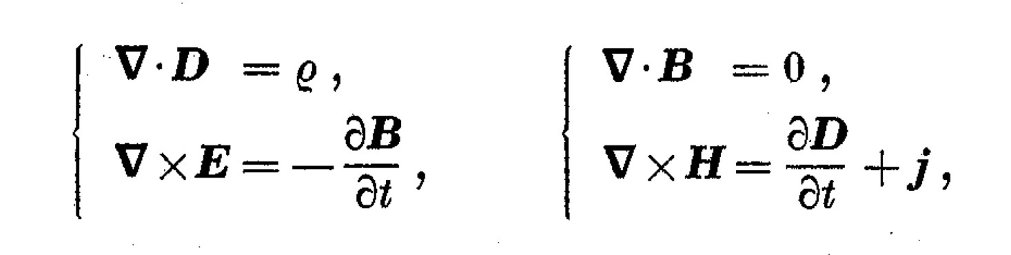
Showing Maxwell’s equations in the relativistic limit using both flux and force (Le Blonde and Le Ballac 1973).

The calculus notation on Maxwell equations can also be simplified to the following (Rousseaux 2005) :-

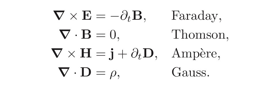
Showing a simplified version of Maxwells Equations (Rousseaux 2013).

As a result of Einstein, the speed of electric and magnetic fields was commonly determined as the speed of light, and this speed would slow down in a medium due to the (electric) permeability (ε) and (magnetic) permittivity (µ). In a vacuum it these values are determined to be 1 and are denoted as ε0 and µ0.

The relationship between forces (E and H) and (D and B) flux are very commonly “simplified” in the modern versions of Maxwell’s equations above by assuming permeability (ε) and permittivity (µ) are 1. So that the assumptions below are made:-

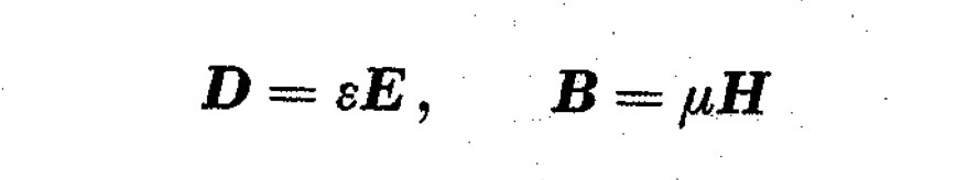
When electric permeability (ε) and magnetic permittivity (µ) are included in modern conventions, the equations show how permeability and permittivity modify the equation. The curl of magnetic force (xH) is modified by the magnetic permittivity (µ) becomes the curl of the electric force (xB). The displacement of electric flux (.D) is modified by the electric permittivity (ε) and becomes the displacement of electric force (.E).

In the relativistic limit, where ε0 and µ0 are included the equations look as follows:-

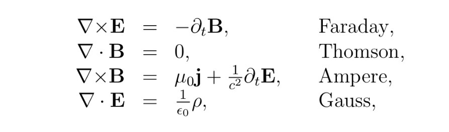
Showing a Maxwells Equations including ε0 and µ0 (Rousseaux 2013).

Slow. moving charges

The expressions in Maxwell’s equations are fully utilised when electromagnetic fields are transmitted from a source. The electromagnetic configuration of transmitting fields was imagined by Maxwell as a feedback loop where energy oscillated between electric and magnetic forces and flux. Later Hertz discovered how a configuration of rapidly moving charges related the transmission of electromagnetic waves. Transmitting electromagnetic waves are relativistic (i.e.the speed of light) and time retardation (i.e. light transmission speed) between the transmitter and receiver need to be taken into account.

A different configuration involving slowly moving charges creates emitting (not transmitting) electric and magnetic fields and does not utilise all the equations in Maxwells equations because the feedback loop is not created. Configurations include motors and dynamos, as well as oscillating charges in brains. This simplification of Maxwells Equations is used by electronic engineers and is known as quasi statics (QE) approximations. The oldest reference to quasi statics is the book by Woodson and Melcher in 1968 (Rousseaux 2013). In treatment of EEG and MEG these limits have been used to simplify equations (Nunez 2006 – appendix B). These engineering simplifications say nothing about the nature of the electromagnetic fields, just that they simplify Maxwells Equations

Quasi-statics is defined as where “the system is small compared with the electromagnetic wavelength associated with the dominant time scale of the problem.” (Jackson 1999). A large range of commonly used electrical equipment fall within the quasi-static regime, including motors, transformers and microelectronics. Quasi-statics are traditionally taught as a simplification of the Maxwell equations, used to help engineers with their calculations on such electronic equipment.

Le Blonde and Le Bellac (1973) showed in quasistatics there are two well defined mutually exclusive (non-relativistic) limits to electrodynamics. One is called the the electric limit and the other the magnetic limit. These limits involve low velocity charges. Where the magnetic field is dominant this leads to the magnetic limit. Where the electric field is dominant this leads to the electric limit. (De Montigny 2005). In addition to the electric and magnetic limits there is a more complex hybrid limit known and the Darwin limit, which utilises more, but not all of Maxwells Equations.

In engineering the following approximations are made using E and B:- (Haus 2000, Castellenos 1998):-

• Electro Quasi Statics (EQS) simplify Maxwell’s equations by neglecting the time-derivative of the magnetic field (∂tB) in Faraday’s law : ∇ × E ≃ 0
• Magneto Quasi Statics (MQS) simplify Maxwell’s equations by neglecting the time-derivative displacement current (∂tE) in Ampere ‘s law : ∇ × B ≃ μ0J
• Darwin’s Approximation simplifies Maxwell’s equations by neglecting “a part of” ∂tE in Ampere law.

Note: EQS and MQS are mutually exclusive limits (Castellenos 1998)

For the engineers looking to simplify Maxwells equations for charges moving at low speeds, the Galilean theory of instantaneous interaction was used because it simplified the calculations point of view. However Le Blonde and Le Bellac (1973) discovered that Galilean Electromagnetism was not just an approximation but real for some interactions. A feature of quasistatics is instantaneous interaction (i.e Galilean relativity) at a distance (Larson 2006). The fields are propagated instantaneously (i.e c → ∞) so there is an absence of time-retardation.

The relationship between different types of fields can be seen in the diagram below. This is defined using a dimensionless parameter α which defines the quasistatic region. Where the wavelength λ = c/T, then the quasistatic limit α ≪ 1 corresponds to L ≪ λ, i.e., the wavelengths are much larger than the characteristic length of interest. Where σ = order of magnitude.

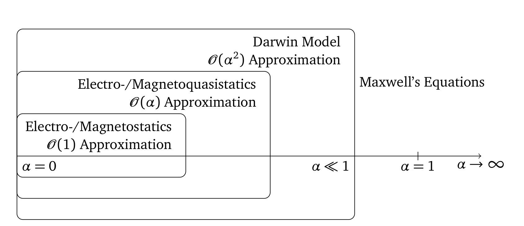
Diagram showing the relations between the various electromagnetic limits (Traub 2014).

The Electric Limit

In the electric limit Isolated electric charges move with low velocities. In the electric limit the motion of an electric field (or its time variation) produces a magnetic field, while a time varying magnetic field does not produce an electric field (Le Blonde and Le Bellac 1973). In the electric limit a magnetic field exists but has no effect (Rousseaux 2006).

These equations describe where isolated charges move with slow velocity.

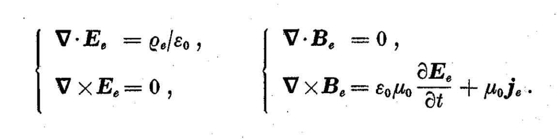
Quasi Electric Maxwell equations (Le Blonde and Le Ballac 1973).

Effectively an electric field (Ee) is generated by electric sources and a magnetic field (Be) that are generated by an electric source. In this limit the magnetic field is not time varying (− ∂tB) and will not create an electric field (∇ × Ee) to couple back onto a magnetic field (Rousseaux 2006).

Faraday’s law of induction does not work. Thus Faradays law of V x E = -∂B/∂t is now V x EE = 0. In the electric limit the electric curl has 0 field in Faraday’s Law.

From an engineering perspective the electric limit is an approximation. “the EQS regime is a good approximation in the interior and vicinity of dielectrics, which might exhibit some losses which takes displacement currents are taken into account and neglects Faradays law” (Kutrtz 2010).

Importantly the magnetic field is incorrectly concluded not to exist by engineers because it does not have any effect. “In the EQS regime, there is no magnetic induction. The EQS regime includes capacitive but not inductive effects because the electric field does not produce a magnetic field. Poyntings Theory shows there is only an electric field. Ampere’s law is not valid.” … “In EQS only the electric field is associated with energy” (Castellenos 1998). EQS involves capacitance features. capacitance is a function only of the geometry of the design and the permittivity of the dielectric material between the plates of the capacitor (Castellenos 1998).

The Magnetic Limit

In the magnetic limit the motion of a magnetic field (or its time variation) produces an electric field while a time varying electric field does not produce a magnetic field (LeBallac 1972). Physically this describes the situation at the macroscopic level where the balance between negative and positive charges. In the magnetic limit there is no displacement current. There can only be stationary currents and no accumulation of charge. The electric field is “non zero” but has no observable effects. (Rousseaux 2006).

These equations describe where magnetic fields charges move with slow velocity.

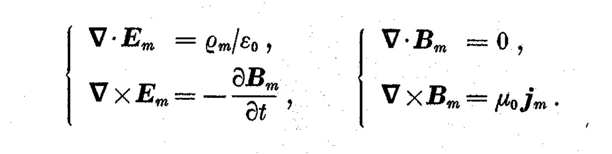
Quasi Magnetic maxwell equations (Le Blonde and Le Ballac 1972)

Effectively an electric field (Em) is generated by magnetic sources and a magnetic field (Bm) is generated by a magnetic source. In the magnetic limit the electric field is not a time varying (1/c2)∂tEe ) (i.e. Maxwells part of the equation) and will not create a magnetic field (∇ x Bm) to couple back onto the electric field. (Rosseaux 2006). In other words there is no induction, whereby an electric field is induced, or generated by a changing magnetic field. This equation only allows stationary currents

From an engineering perspective “The MQS regime good approximation in the interior and vicinity of good conductors, which takes Faradays laws into account but neglects displacement currents. In the MQS regime, only stationary currents are allowed and these currents cannot explain time changes in the charge density ρ.” (Kutrtz 2010).

In engineering the electric field is incorrectly concluded not to exist because it has not effect. “The MQS regime includes inductive but not capacitive effects, because only stationary electric fields are allowed and these do not change the charge density. Poyntings Theory shows there is no magnetic field. Ampere’s law is valid. … In MQS only the magnetic field has energy. (Castellenos 1998)

Super luminal Electric and Magnetic Fields

LeBlonde and Le Ballac (1973) warned that defining c → ∞ in the quasi static limits was bound to produce questionable results. Instead the value of c should come from the equations.

In a MKSA system the initially <<independent>> coefficients ε0 µ0 turn out to be related by the formula ε0 µ0 c²=1. This is sufficient to show that Maxwell’s equations cannot have a nonrelativistic limit (c → ∞) where ε0 µ0 both remain finite. The possibility of keeping one of them finite, at will, implies the existence of the two Galilean limits. In fact the following prescription yields the <<magnetic>> limit: express the relativistic theory in terms of the usual E and B keeping µ0 but eliminating ε0 then let c go to infinity. To obtain the <<electric>> limit express the relativistic theory in terms of E keeping ε0 but eliminating µ0. – Le Blond and Le Ballac 1973

In otherwords if where ε0 < 1 then superluminal fields in the electric limit, and where µ0 < 1 then superluminal fields in the magnetic limit.

The Darwin Limit

A third hybrid limit called the Darwin limit has also been shown to exist for higher velocity charges. The Darwin limits neglects the transverse, but not longitudinal, electric field

“for some problems, e.g., the simulation of charged particles when no high frequency phenomenon or no rapid current change occurs, it is possible to use some simplified model which approximates Maxwell’s equations and can be solved more economically. The Darwin model is such a simplified model. ” (Liao 2008)

Degond and Raviart (1992) decomposed the electric field E into the sum of its transverse component ET and longitudinal component EL, where ET is divergence free and EL is curl free. The Darwin model is obtained by neglecting ∂Et/∂t. In otherwords the transverse electric field that creates the solenoidal part of amperes law is neglected. In MQS and Darwin there is a contribution to the electric field due to magnetic induction (from ∂B/∂t in Faraday’s law). (Castellenos 1998)

Raviart (1994) used Helmholtz decomposition to show the electric field is composed of a longitudinal field (EL) and transverse (ET) field.

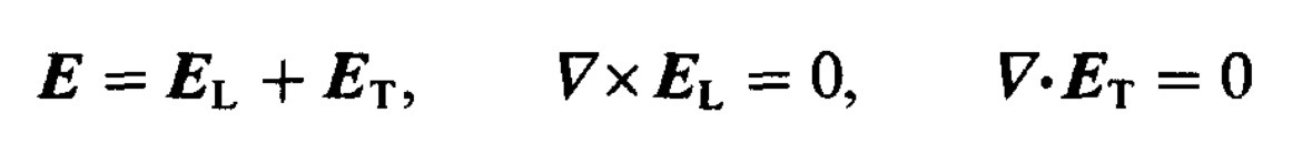
Equation showing the decomposition of the electric and transverse fields in the Darwin limit (Raviart 1994). Where EL is curl free and ET is divergence free

The Helmholtz decomposition then produces the following set of separate equations.

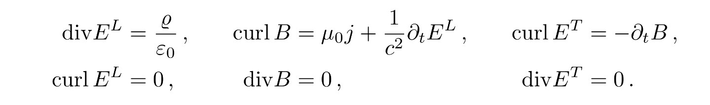
This led to the following conclusion by Bauer (2018). “Prior to Maxwell there were two independent div[ergent] curl systems. In Maxwell’s equations there are two curl div[ergent] systems where the results of one feed into the source of the next. In Darwin there are three div[ergent] curl systems where the results fed into the next one.” – Bauer 2018.

From an engineering perspective “The Darwin model includes both capacitive and inductive effects, but there is no radiation and uses the Coloumb Gauge. No interactions are instantaneous (Larsson 2006). Poytings theorem shows there is both electric and magnetic energy but electric energy only shows the Coloumb part of the field. Within the Darwin model the Biot-Savart law is valid and Ampere’s law is not. ” (Castellenos 1998).

Larson (2006) draws some important conclusions. First that the Darwin limits are able to create feedback and thereby oscillations but not radiation. “An important qualitative difference between EQS and MQS on the one side and Darwin’s model on the other is the possibility of natural resonances in the latter. (Larson 2006) A qualitatively new feature of Darwin’s model (as opposed to MQS or EQS) is the possibility of resonance but there is no radiation and the interactions are instantaneous.

Larson (2006) also concludes that the oscillations could include energy oscillating between electric and magnetic energy. “Since the Darwin model includes both capacitive and inductive phenomena it may in principle be used to model systems where the energy oscillates between the electric and magnetic fields. but the frequency must be low enough not to violate the quasistatic assumption.”,

Finally, Larson (2006) recognised that “The use of two complementary quasistatic models in the same physical system is clearly a complicating feature if we like to model the whole system numerically. We would then have to divide the whole spatial region into EQS and MQS subregions with appropriate continuity conditions at the interfaces. A better alternative may be to use the Darwin model which embrace all the physics contained in EQS and MQS, still being quasistatic.”

Conclusion

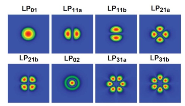
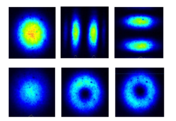
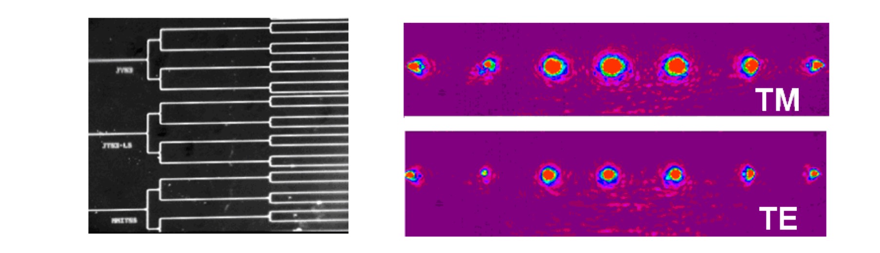
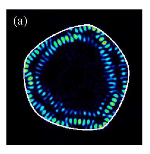
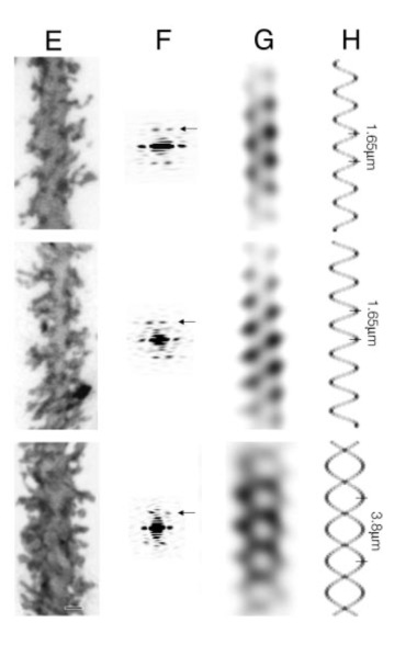
It is true to say that electric and magnetic fields in the brain result from slow moving, low energy ions. It is therefore true to say that quasi static electric, magnetic and Darwin quasi static fields probably exist in the brain. It is also true that the “non-casual” fields from the ions have curl reflecting the wavelengths on light transmitted from ions, It is also true to say that the wavelengths of the ions in the brain are similar to the (diametric) geometry of brain cells and could therefore create guided wave modes as explained in previous posts. Importantly these Galilean quasi static fields, could create guided wave modes and could interact.

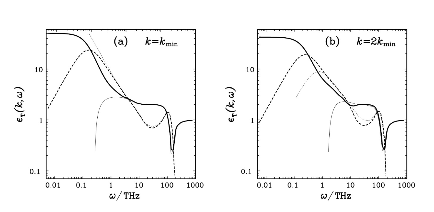
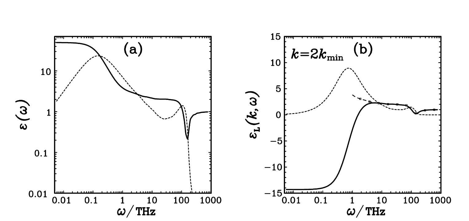
Further is has been shown (Omelyan 1999 a,b) that complex dielectric functions resulting from the oscillations of water reduces the permeability (ε) in the transverse (T) and longitudinal (L) direction differently in water. In particular the permeability of water in a longitudinal direction is greatly reduced to wavelengths including those of ions in the brain. These oscillations would effect fields in the Darwin limit which also function differently in the longitudinal and transverse direction.

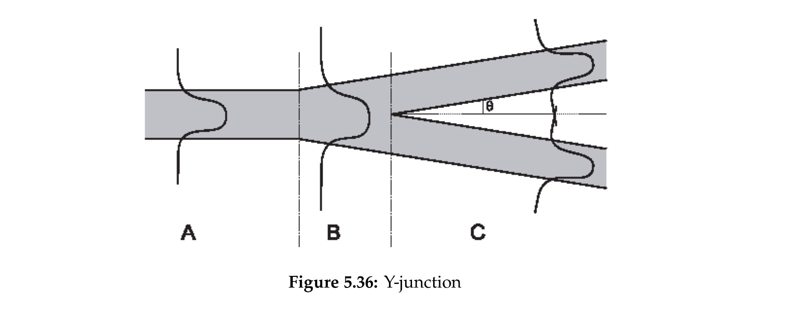
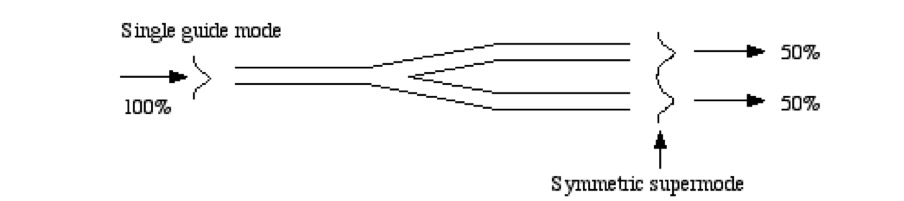
Oscillations in water could provide a means of creating switches, wires and waveguides in water for ion sourced fields. The longitudinal properties of oscillating water and longitudinal fields in Darwinian quasi statics are complimentary. The ability of oscillating water to drastically change permeability means water can change the curl and divergence of quasi static electric and magnetic fields enabling ‘calibrated’ (custom) waveguide and modes.

Complex dielectrics in Water

The purpose of this post is to look at the behaviour of water under “complex” fields to better iunderstand how water behaves in neurons. Complex means both oscillating (“static”) fields (aka. wave-vector) and electromagnetic (“transmitted”) fields (aka. frequency-vector).

Previous posts have looked at static electric fields, oscillating electric fields in free space, the absorption and dispersion of different electromagnetic wavelengths in water and the dielectric constant of water at interfaces. However previous posts have not looked at the more realistic case of oscillating fields (wave-vector dependent dielectric function) and electromagnetic fields (frequency-dependent dielectric function) at charged interfaces in water at the same time. The reason this is significant is that electric charges in the brain oscillate in water creating oscillating fields and the radiation of (slow) electromagnetic waves in water is effected by oscillating fields and charged interfaces.

However while more realistic this is not accurate as brain waves do not involve traditional transmitted electro-magentic fields, rather fields emitted from slow-moving ions. Dealing with thi requires a better understanding of the theory of slow moving electric fields.

The frequency and wave-vector-dependent dielectric function, ε(q,w), is a complex function, which describes the screening and absorption of a field which varies in both space and time in a dielectric medium. This complex dielectric function measures the response to weak external longitudinal or transverse fields of the energy of an accelerating charged particle which varies with space and time and the time-dependent collective excitation waves (density fluctuations) of the electronic “fluid” (plasmon modes).

When an electric field (E) is applied to water the dipoles increase in alignment and there said to be an increase in permittivity. Permittivity is a measure of how easily polarisation (alignment) occurs. When the electric field weakens the dipoles unalign, biased on external electric fields. The speed of aligning and unaligning is known as polorization and relaxation time. It has been hypothesised in a previous post that dipole de-alignment is cased by external electric fields, such as action potentials and mechanical stirring by neurofilament arms.

If the speed of oscillations polorizing the dielectric is faster than the speed of relaxation the water is more likely to stay polorised. Where the water exists near a charged surface then the water has a much higher likely hood of being polorized and a lower likelyhood of being depolarised. This would mean the electric field conducts better through the water near charged interfaces.

In addition the alignment of water dipoles promotes the long range migration of protons (Gabriel 1984, Tessie 1996).

Longitudinal and Transverse Permittivity

Water has ansiotrophic dielectric properties. Anisotropy of an object or substance means having a physical property which has a different value when measured in different directions. An example is wood, which is stronger along the grain than across it. Anisotropy is essential to understand the behaviour or electric fields in water. “The general trend in experiments, which shows that both parallel and perpendicular components of the dielectric function are essential in order to reproduce experimental findings.” (Gekle 2016).

Omelyan (2016) examined the electric and magnetic fields using both the TIP4P water model and the Interaction Site Model (IS), and found the permeability differed between the transverse (T) and longitudinal (L) direction.

Omelyan found that the point dipole (PD) approach was valid for describing the frequency dependence of the dielectric constant at very small wavenumbers only. The point dipole (PD) approach, assumed charged sites for each molecule were replaced by a point dipole, located in the molecular centre of mass.

A different model used was a more realistic interaction site (IS) models where intermolecular potentials are modelled as the “sum of pairwise additive site-site terms” and do not take into account internal degrees of freedom such as electronic polarisation and intramolecular vibrations. IS models were able to reproduce experimental results in a more satisfactory way.

Omelyan (2016) predictions did not include the secondary effect of dynamical magnetic fields of moving charges which would create stronger polarization effects and spatial forms. Omelyan (1999) assumed a 6.7ps is the relaxation time in bulk water.

Transverse and Longitudinal Fields

Omelyan calculated the permeability (ε) in the transverse (T) and longitudinal (L) direction as εT and εL.

In the diagrams below the solid lines represents real dielectric component (permittivity) and the dashed line imaginary dielectric component. Where the real component refers to the slowing down of the electromagnetic wave with increasing frequency, from the constant static point. The imaginary permittivity component refers to the loss of energy.

The model assumed a “simple forced damped oscillator… the real component describes the phase lag between the driving and response frequency (slowing down of light in a material, described by the refractive index) and the imaginary component is the damping factor (loss of energy or absorption of light, described by the absorption co-efficient” (Omelyan 2016).

Transverse Oscillations

The diagram below shows the predicted electric transverse (εT) permittivity of water for low oscillations between the minimum and 2k (Omelyan 1999a).

The wavelength of visible light of 390 to 700 nm corresponds to 430THz to 770THz and the oscillations in the brain are between min and 200.

At visible light wavelengths and brain oscillation levels the longitudinal real dielectric constant drops below 1 and the transverse imaginary dielectric constant (losses) drops towards zero.

Graph showing the predicted transverse (ε(w)) permitivity of water (Omelyan 1999a)

Longitudinal Oscillations

The diagram below shows the predicted electric longitudinal (εT) permittivity of water for low oscillations between minimum and 2k (Omelyan 1999b).

At visible light wavelengths and minimum oscillation levels the longitudinal real dielectric constant drops below 1 and the longitudinal imaginary dielectric constant (losses) drops to around zero. When the oscillations rise both the longitudinal real complex dielectric constant drops towards zero.

Graph showing the predicted longitudinal (ε(w)) permittivity of water (Omelyan 1999b)

Nano confined biological water

Biological water exhibits much lower dielectric relaxation (i.e. real dielectric permittivity) than in bulk water (1 trillionth of a second = 10^-12s,). because in bulk water free moving water contributes to the relaxation process.

Biological water is complex, so measurements are needed. The table below shows measured dielectric relaxation in the complex biomolecular systems ranging from 20 nano seconds to 10 picoseconds.

Table from Nandi (1997) showing relaxation time in bio-water.

Li (2018) found the relaxation time of nano-confined water is in the range 0.1 − 0.0001 s, intrinsically 0.06s, which is orders of magnitude longer than that of bulk water. (one trillionth of a second).

This post shows that the dielectric constant of water could be changed by brain oscillations to effect electric and magnetic fields in the same time scales as action potentials. This raises the possibility that oscillating ions changing the state of water could create temporary electrical pathways.